3. Vegetation Classification: Dam Building Material Preferences

Figure 2 shows how the LANDFIRE land cover data can be classified in terms of its suitability as beaver dam building material.

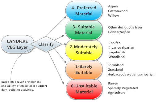
Figure 2. Diagram showing LANDFIRE land cover data classification for the beaver dam capacity model

Task 1: Classify LANDFIRE Land Cover Data

• Step 1: Make a copy of your vegetation type layer (e.g. US_120evt) as a new raster (we suggest using *.img or *.tif; e.g. LANDFIRE_EVT.img) in the same coordinate system as your drainage network layer.

• Step 2: Load your vegetation type raster and add a field called “VEG_CODE” representing dam-building material preferences (0-4) (Table 1).

• Step 3: Classify the VEG_CODE field according to its suitability as a dam building material. Example classifications are shown below.

Table 1. Suitability of LANDFIRE Land Cover as Dam-building Material

Suitability	Description	LANDFIRE Land Cover Classes
0	Unsuitable Material	Agriculture, roads, barren, non-vegetated, or sparsely vegetated
1	Barely Suitable Material	Herbaceous wetland/riparian or shrubland, transitional herbaceous, or grasslands
2	Moderately Suitable Material	Introduced woody riparian, woodland/conifer, or sagebrush
3	Suitable Material	Deciduous upland trees, or aspen/conifer
4	Preferred Material	Aspen, cottonwood, willow, or other native woody riparian

Below is an example that you can either download or use as a rough guide (alternatively download the CSV file: EVT_VEG_Classification.csv or BPS_VEG_Classification ). We suggest you consider the classification carefully for those vegetation types that end up in your riparian areas, but remember that the majority of categories occur well outside the riparian corridor and are not critical in this analysis. Columns A through Q are those you will find in the raster attribute table. Column R is the ‘VEG_CODE’ column which is classified with a 0 through 4 categorical suitability class.

Below is a video that details the process used in step 3 to classify the LANDFIRE vegetation data in terms of dam building suitability for beaver.

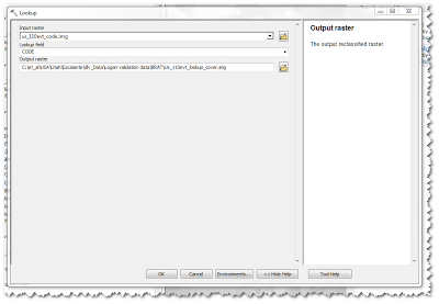
• Step 4: To create a raster that we can calculate zonal statistics from, we need a raster that has our new ‘‘VEG_CODE’ as its value field. Use the “Lookup” command to generate a new raster (e.g. 120evt_Look_Up_Code.img) with “VEG_CODE” as the “lookup” field. Perform this step twice, once for Existing (US 120 evt) vegetation and once for Potential (US 120 bps) vegetation.

• Step 5: Perform Zonal Statistics on both the 30 m and 100 m buffers. Using the “Zonal Statistics” command (ArcToolbox under Spatial Analyst Tools -> zonal).

• • Statistics type: Mean
  • Conduct this step a total of four times.

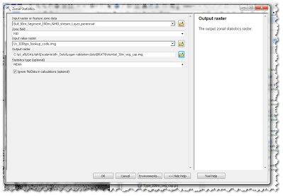
• 1st: Use Buf_100m_Seg_300m_NHD_Perennial as the zone data. Use the LANDFIRE land cover (Existing) Us_120evt_Look_Up_Code.img as the input value raster.
• 2nd: Use Buf_30m_Seg_300m_NHD_Perennial as the zone data. Use the LANDFIRE land cover (Existing) Us_120evt_Look_Up_Code.img as the input value raster.
• 3rd: Use Buf_100m_Seg_300m_NHD_Perennial as the zone data. Use the LANDFIRE land cover (Potential) Us_120bps_Look_Up_Code.img as the input value raster.
• 4th: Use Buf_30m_Seg_300m_NHD_Perennial as the zone data. Use the LANDFIRE land cover (Potential) Us_120bps_Look_Up_Code.img as the input value raster.

Below we illustrate how you can use Zonal Statistics to clip and average your classified vegetation raster into your buffered areas:

<- Back to Step 2 Ahead to Step 4 ->